Chapter 2 Review of Basic Statistics

library(rio); library(psych); library(Hmisc); library(ggplot2); library(reshape2); library(QuantPsyc); library(MASS); library(lavaan)

2.1 Calculating Variance and Covariance

2.1.1 Covariance

population: $σ_{XY} = \frac{\sum (X - μ_{X}) (Y - μ_{Y})}{N_{p o p}}$ sample: $s_{X Y} = {\hat{σ}}_{X Y} = C o v (X, Y) = \frac{\sum (X - \bar{X}) (Y - \bar{Y})}{(n - 1)}$

2.1.2 Correlation

population: $ρ_{XY} = \frac{σ_{XY}}{\sqrt{{σ_{X}}^{2} {σ_{Y}}^{2}}}$

sample: $r_{XY} = {\hat{ρ}}_{XY} = \frac{C o v (X, Y)}{\sqrt{{s_{X}}^{2} {s_{Y}}^{2}}}$

2.1.3 Using Matrix Algebra

Suppose we have a 5 by 2 data matrix X (2 variables and 5 participants, for example). $=$

First, we calculate the deviation score matrix $X_{d}$ .

$X_{d} = X - \bar{X} = [\begin{matrix} 1 & 3 \\ 4 & - 5 \\ 1 & 7 \\ 3 & 2 \\ 7 & - 1 \end{matrix}] - [\begin{matrix} 3.2 & 1.2 \\ 3.2 & 1.2 \\ 3.2 & 1.2 \\ 3.2 & 1.2 \\ 3.2 & 1.2 \end{matrix}] = [\begin{matrix} - 2.2 & 1.8 \\ 0.8 & - 6.2 \\ - 2.2 & 5.8 \\ - 0.2 & 0.8 \\ 3.8 & - 2.2 \end{matrix}]$

Next, we multiple the transpose of $X_{d}$ ( ${X_{d}}^{^{'}}$ ) by $X_{d}$ itself using matrix operations. We will get the deviation SSCP (sums of squares and cross products) matrix.

Deviation SSCP matrix:
${X_{d}}^{'} X_{d} = \sum x_{i} x_{j} = [\begin{matrix} \sum x_{1}^{2} & \sum x_{1} x_{2} \\ \sum x_{2} x_{1} & \sum x_{2}^{2} \end{matrix}] = [\begin{matrix} 24.8 & - 30.2 \\ - 30.2 & 80.8 \end{matrix}]$ (Note: Lower case $x_{i}$ ’s represent deviation scores.)

Since variance of of the first variable $X_{1}$ is $\frac{1}{N - 1} \sum x_{1}^{2}$ and the covariance between $X_{1}$ and $X_{2}$ is $\frac{1}{N - 1} \sum x_{1} x_{2}$ , the variance and covariance matrix (usually denoted by S) can be obtained by multiplying $\frac{1}{N - 1}$ to the deviation score SSCP:

Variance and Covariance matrix: $S = \frac{1}{5 - 1} [\begin{matrix} 24.8 & - 30.2 \\ - 30.2 & 80.8 \end{matrix}] = [\begin{matrix} 6.2 & - 7.55 \\ - 7.55 & 20.2 \end{matrix}]$

Sample Covariance Matrix S

Sample Correlation R

Elements in sample covariance matrix divided by $s_{i} s_{j}$ would result in the sample correlation matrix.

Elements in sample correlation matrix multiplied by $s_{i} s_{j}$ would result in the sample covariance matrix.

2.2 Use R for Basic Statistics

2.2.1 Import and export data

mydata <- import("data/example.sav")
# head(mydata) # view first 6 observations

export(mydata, file = "data/dataset_example.csv")
export(mydata, file = "data/dataset_example.xlsx")

2.2.2 Several functions for basic data management

names(mydata)[names(mydata) == "ITSEX"] <- "gender" #rename a variable
names(mydata)[names(mydata) == "BSMMAT01"] <- "math" #rename another variable for math score
names(mydata)[names(mydata) == "BSBGHER"] <- "resource" #education resource
names(mydata)[names(mydata) == "BSBGSCM"] <- "confidence" #confidence in math
names(mydata)[names(mydata) == "BSBGSVM"] <- "value" #valuing math
names(mydata)[names(mydata) == "BSBGSSB"] <- "belonging" #sense of belonging
var <- c("gender", "math", "resource", "confidence", "value", "belonging")
dat1 <- mydata[, var] #subset data
dat2 <- na.omit(dat1) #listwise deletion
dat1$gender_c <- factor(dat1$gender) #create a categorical variable for `gender`
levels(dat1$gender_c) <- c("f", "m") #change levels for `gender` variable

2.2.3 Some descriptive statistics

summary(dat1) 
table(dat1$gender_c) #compute frequencies for categorical variables
psych::describe(dat1) #compute descriptives for quantitative variables. Need to install and load the `psych` package
attach(dat1) # save some typing. Alternatively, `math <- dat1$BSMMAT01` to create a separate vector.

## The following object is masked _by_ .GlobalEnv:
## 
##     gender

mean(math, na.rm = TRUE)
median(math, na.rm = TRUE)
var(math, na.rm = TRUE)
sd(math, na.rm = TRUE)
quantile(math, na.rm = TRUE)
detach(dat1)

2.2.4 Check normality

shapiro.test(dat1$math)

You got an error message.
The Shapiro-Wilk test is for small to moderate samples.

set.seed(12345) #for reproducibility
selected <- sample(nrow(dat1), 100) #randomly selection 100 numbers from 1 through the sample size
dat1_small <- dat1[selected,] #create a smaller dataset of 100 students
shapiro.test(dat1_small$math)

## 
##  Shapiro-Wilk normality test
## 
## data:  dat1_small$math
## W = 0.97872, p-value = 0.1056

2.2.5 Check linearity

plot(dat2$confidence, dat2$math)
abline(lm(math ~ confidence, data =dat2), col = "red")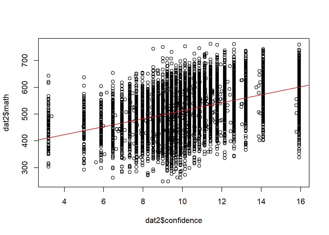

2.2.6 Pearson’s product moment correlation

Correlation between two variables, hypothesis test, and confidence interval.

cor.test(dat1$resource, dat1$math)

## 
##  Pearson's product-moment correlation
## 
## data:  dat1$resource and dat1$math
## t = 42.923, df = 10116, p-value < 2.2e-16
## alternative hypothesis: true correlation is not equal to 0
## 95 percent confidence interval:
##  0.3759021 0.4088708
## sample estimates:
##       cor 
## 0.3925126

All pairwise correlations.

cor(dat1[,var], use = "pairwise.complete.obs") #for numeric variables only; "gender" is still a numeric variable!

##                  gender       math   resource confidence      value   belonging
## gender      1.000000000 0.01305597 -0.0281559  0.0719095 0.03690314 0.007168246
## math        0.013055968 1.00000000  0.3925126  0.4280530 0.16511215 0.221113350
## resource   -0.028155898 0.39251256  1.0000000  0.1512655 0.10208246 0.152041678
## confidence  0.071909498 0.42805300  0.1512655  1.0000000 0.37535602 0.280950896
## value       0.036903141 0.16511215  0.1020825  0.3753560 1.00000000 0.366637734
## belonging   0.007168246 0.22111335  0.1520417  0.2809509 0.36663773 1.000000000

round(cor(dat1[,var], use = "pairwise.complete.obs"), 2) #round to 2 decimal places

##            gender math resource confidence value belonging
## gender       1.00 0.01    -0.03       0.07  0.04      0.01
## math         0.01 1.00     0.39       0.43  0.17      0.22
## resource    -0.03 0.39     1.00       0.15  0.10      0.15
## confidence   0.07 0.43     0.15       1.00  0.38      0.28
## value        0.04 0.17     0.10       0.38  1.00      0.37
## belonging    0.01 0.22     0.15       0.28  0.37      1.00

Correlations and significance levels for the correlation matrix. Need to install and load the Hmisc package. Need to coerce from dataframe to matrix to get both a correlation matrix and p-values.

install.packages("Hmisc")
library(Hmisc)

df <- as.matrix(dat1[,var]) # numeric variables only
rcorr(df)

##            gender math resource confidence value belonging
## gender       1.00 0.01    -0.03       0.07  0.04      0.01
## math         0.01 1.00     0.39       0.43  0.17      0.22
## resource    -0.03 0.39     1.00       0.15  0.10      0.15
## confidence   0.07 0.43     0.15       1.00  0.38      0.28
## value        0.04 0.17     0.10       0.38  1.00      0.37
## belonging    0.01 0.22     0.15       0.28  0.37      1.00
## 
## n
##            gender  math resource confidence value belonging
## gender      10217 10217    10117      10052 10014     10111
## math        10217 10221    10118      10053 10015     10112
## resource    10117 10118    10118      10017  9978     10073
## confidence  10052 10053    10017      10053 10010     10035
## value       10014 10015     9978      10010 10015      9998
## belonging   10111 10112    10073      10035  9998     10112
## 
## P
##            gender math   resource confidence value  belonging
## gender            0.1870 0.0046   0.0000     0.0002 0.4711   
## math       0.1870        0.0000   0.0000     0.0000 0.0000   
## resource   0.0046 0.0000          0.0000     0.0000 0.0000   
## confidence 0.0000 0.0000 0.0000              0.0000 0.0000   
## value      0.0002 0.0000 0.0000   0.0000            0.0000   
## belonging  0.4711 0.0000 0.0000   0.0000     0.0000

2.3 Use R for Graphing Data

2.3.1 Use `plot()`

Use browseURL("https://datalab.cc/rcolors") to view different colors and methods to refer to them. Use ?palette for palettes in R; use palette() for current palette

plot(dat1$value, dat1$math)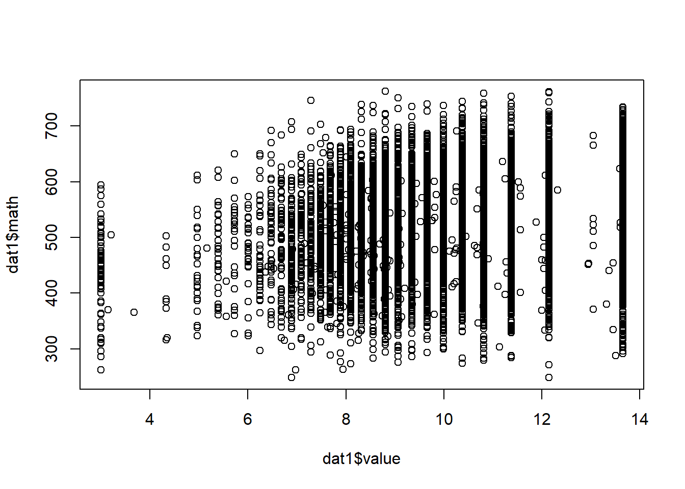

plot(dat1$value, jitter(dat1$math)) # add some random noise to Y

plot(dat1$value, jitter(dat1$math), xlab = "Valuing Math", ylab = "Math Score") # change labels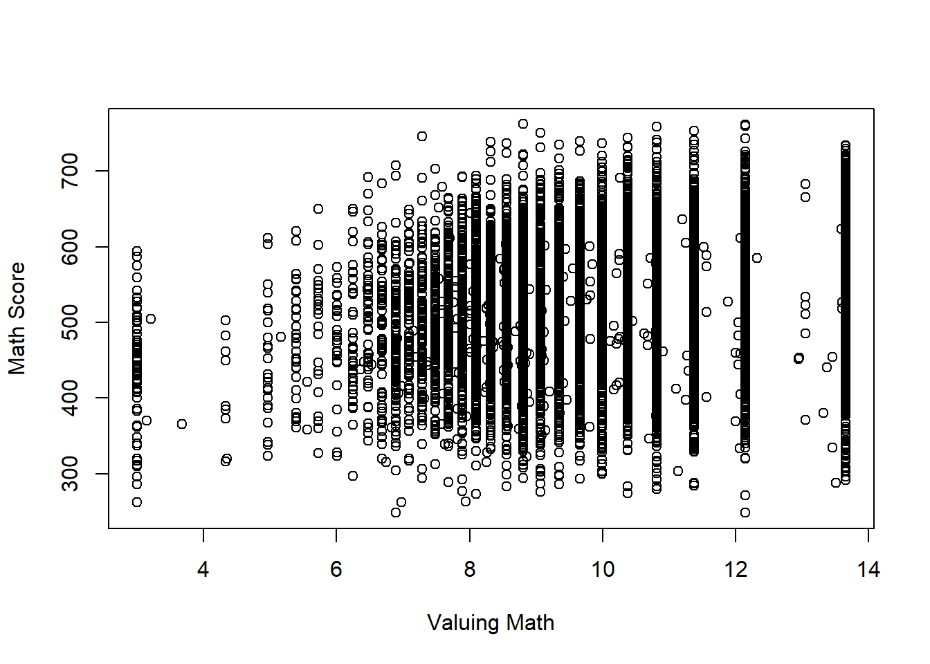

plot(dat1$value, jitter(dat1$math), xlab = "Valuing Math", ylab = "Math Score", col = "red") # change color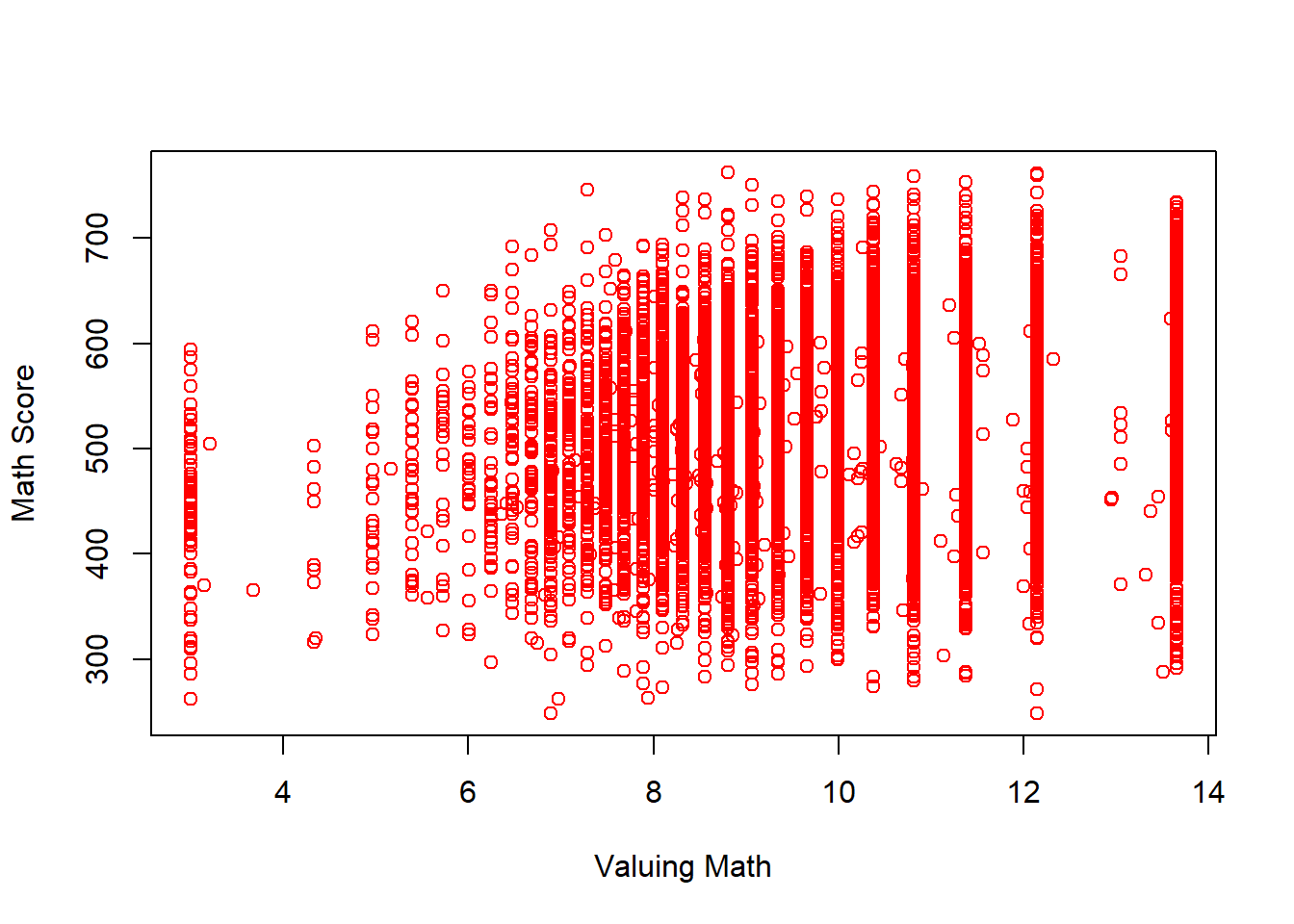

2.3.2 Use `ggplot2` package

Read Chapter 4 of textbook Field, Miles, Field (2012).

install.packages("ggplot2")
library(ggplot2)

ggplot(dat1, aes(math)) +
  theme(legend.position = "none") +
  geom_histogram(aes(y = ..density..), colour = "black", fill = "white") + 
  labs(x = "Math", y = "Density") + 
  stat_function(fun = dnorm, args = list(mean = mean(dat1$math, na.rm = TRUE), sd = sd(dat1$math, na.rm = TRUE)), colour = "red", size = 1)

## `stat_bin()` using `bins = 30`. Pick better value with `binwidth`.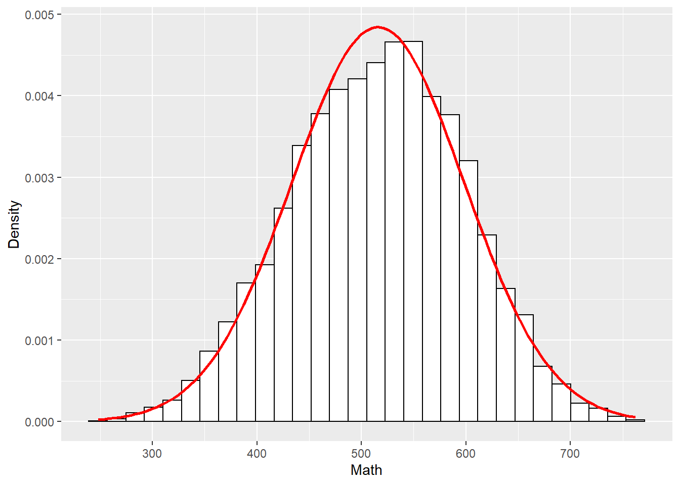

2.4 Use R to Graph a Correlation Matrix

2.4.1 Use `plot()`

plot(dat1[,var])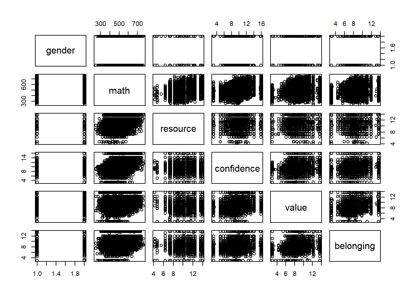

2.4.2 Use `ggplot()`

install.packages("reshape2")
library(reshape2)

(cor_matrix <- cor(dat1[,var], use = "pairwise.complete.obs"))

##                  gender       math   resource confidence      value   belonging
## gender      1.000000000 0.01305597 -0.0281559  0.0719095 0.03690314 0.007168246
## math        0.013055968 1.00000000  0.3925126  0.4280530 0.16511215 0.221113350
## resource   -0.028155898 0.39251256  1.0000000  0.1512655 0.10208246 0.152041678
## confidence  0.071909498 0.42805300  0.1512655  1.0000000 0.37535602 0.280950896
## value       0.036903141 0.16511215  0.1020825  0.3753560 1.00000000 0.366637734
## belonging   0.007168246 0.22111335  0.1520417  0.2809509 0.36663773 1.000000000

(melt_cor_matrix <- melt(cor_matrix))

## Warning in melt(cor_matrix): The melt generic in data.table has been passed a matrix and will attempt to redirect to the relevant
## reshape2 method; please note that reshape2 is deprecated, and this redirection is now deprecated as well. To continue using melt methods
## from reshape2 while both libraries are attached, e.g. melt.list, you can prepend the namespace like reshape2::melt(cor_matrix). In the
## next version, this warning will become an error.

##          Var1       Var2        value
## 1      gender     gender  1.000000000
## 2        math     gender  0.013055968
## 3    resource     gender -0.028155898
## 4  confidence     gender  0.071909498
## 5       value     gender  0.036903141
## 6   belonging     gender  0.007168246
## 7      gender       math  0.013055968
## 8        math       math  1.000000000
## 9    resource       math  0.392512564
## 10 confidence       math  0.428053003
## 11      value       math  0.165112146
## 12  belonging       math  0.221113350
## 13     gender   resource -0.028155898
## 14       math   resource  0.392512564
## 15   resource   resource  1.000000000
## 16 confidence   resource  0.151265456
## 17      value   resource  0.102082458
## 18  belonging   resource  0.152041678
## 19     gender confidence  0.071909498
## 20       math confidence  0.428053003
## 21   resource confidence  0.151265456
## 22 confidence confidence  1.000000000
## 23      value confidence  0.375356020
## 24  belonging confidence  0.280950896
## 25     gender      value  0.036903141
## 26       math      value  0.165112146
## 27   resource      value  0.102082458
## 28 confidence      value  0.375356020
## 29      value      value  1.000000000
## 30  belonging      value  0.366637734
## 31     gender  belonging  0.007168246
## 32       math  belonging  0.221113350
## 33   resource  belonging  0.152041678
## 34 confidence  belonging  0.280950896
## 35      value  belonging  0.366637734
## 36  belonging  belonging  1.000000000

ggplot(data = melt_cor_matrix,
       aes(x = Var1, y = Var2, fill = value)) + geom_tile()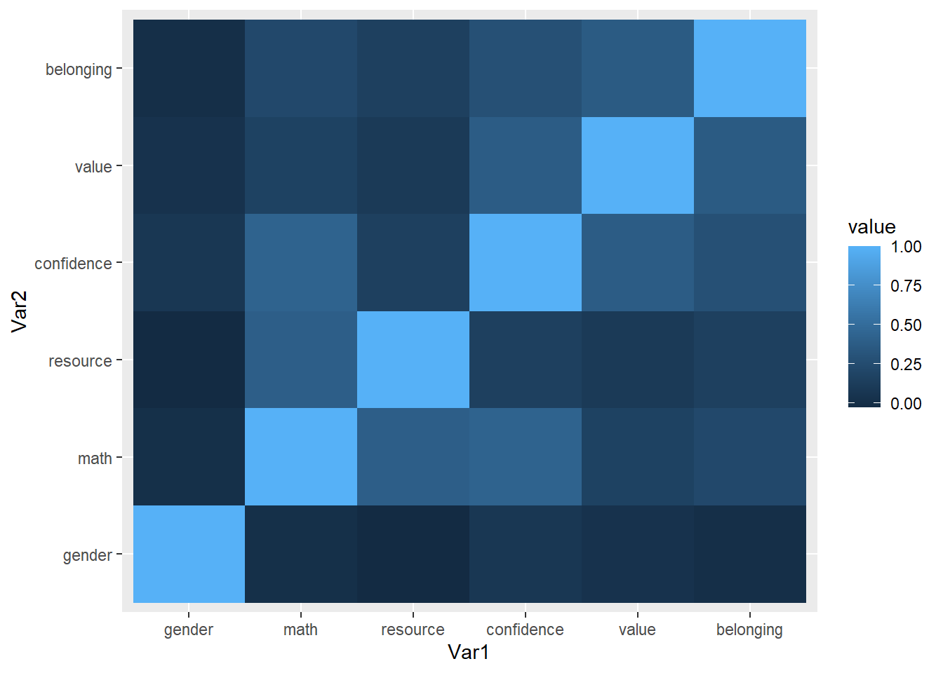

2.5 Use R to Generate Random Data

2.5.1 Sampling distribution

Generate data.

size <- 50
sample_means <- NULL
for (i in 1:1000) {
  samp <- rnorm(size, 10, 5)
  sample_means[i] <- mean(samp)
}

Calculate the mean and SD of the sampling distribution.

mean(sample_means) # population mean is 10

## [1] 10.007

sd(sample_means)  # SD of the sampling distribution

## [1] 0.708293

Use hist() to graph the sample means for sampling distribution.

hist(sample_means, breaks = 50, main = "N= 50", xlab = "Sample Means", probability = TRUE)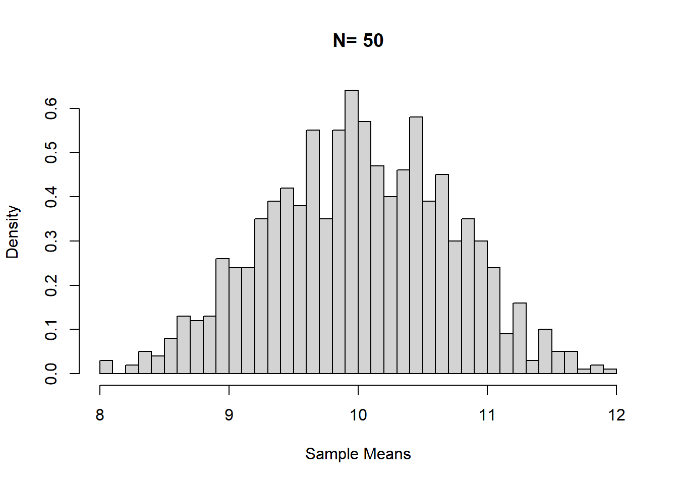

Use ggplot() to graph the sample means for sampling distribution.

df_sample_means <- data.frame(i = 1:1000, sample_means) # data for ggplot has to be a data frame.
ggplot(df_sample_means, aes(x = sample_means)) +
  geom_histogram(aes(y = ..density..), colour = "black", fill = "white") + 
  labs(x = "Sample Means", y = "Density") + 
  stat_function(fun = dnorm, args = list(mean = mean(df_sample_means$sample_means, na.rm = TRUE), sd = sd(df_sample_means$sample_means, na.rm = TRUE)), colour = "red", size = 1)

## `stat_bin()` using `bins = 30`. Pick better value with `binwidth`.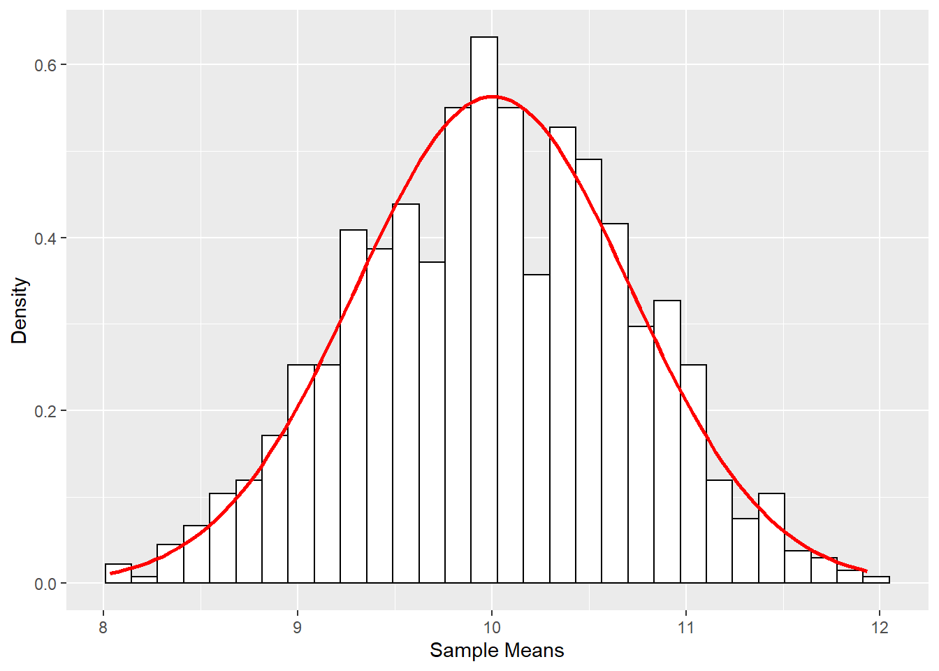

2.5.2 Simulate data from a model

####Simulate data based on a regression model####

Simple Linear Regression with 0.7 correlation between x and y

x <- rnorm(1000, 10, 2)
Zx <- scale(x)
Zy <- .7*Zx + rnorm(1000, 0, sqrt(1-(.7^2)))
y <- 3*Zy + 5
dat1 <- data.frame(x,y)
cor(x,y)

##          [,1]
## [1,] 0.693814

summary(lm(Zy ~ 0 + Zx))

## 
## Call:
## lm(formula = Zy ~ 0 + Zx)
## 
## Residuals:
##      Min       1Q   Median       3Q      Max 
## -1.93796 -0.49421 -0.01251  0.51644  2.37284 
## 
## Coefficients:
##    Estimate Std. Error t value Pr(>|t|)    
## Zx  0.71276    0.02341   30.44   <2e-16 ***
## ---
## Signif. codes:  0 '***' 0.001 '**' 0.01 '*' 0.05 '.' 0.1 ' ' 1
## 
## Residual standard error: 0.74 on 999 degrees of freedom
## Multiple R-squared:  0.4813, Adjusted R-squared:  0.4807 
## F-statistic: 926.8 on 1 and 999 DF,  p-value: < 2.2e-16

summary(lm(y ~x))

## 
## Call:
## lm(formula = y ~ x)
## 
## Residuals:
##     Min      1Q  Median      3Q     Max 
## -5.7646 -1.4334  0.0117  1.5986  7.1678 
## 
## Coefficients:
##             Estimate Std. Error t value Pr(>|t|)    
## (Intercept) -5.85417    0.36189  -16.18   <2e-16 ***
## x            1.07541    0.03533   30.44   <2e-16 ***
## ---
## Signif. codes:  0 '***' 0.001 '**' 0.01 '*' 0.05 '.' 0.1 ' ' 1
## 
## Residual standard error: 2.221 on 998 degrees of freedom
## Multiple R-squared:  0.4814, Adjusted R-squared:  0.4809 
## F-statistic: 926.3 on 1 and 998 DF,  p-value: < 2.2e-16

QuantPsyc::lm.beta(lm(y ~x))

##        x 
## 0.693814

Multiple Linear Regression with with known population standardized regression coefficients

x1 <- rnorm(1000, 10, 2)
x2 <- rnorm(1000, 5, 1)
x3 <- x1*x2
Zx1 <- scale(x1)
Zx2 <- scale(x2)
Zx3 <- scale(x3)
Zy <- .7*Zx1 + .5*Zx2 + 2*Zx3 + rnorm(1000, 0, sqrt(1-(.49+.25+.04)))
y <- 3*Zy + 5
dat2 <- data.frame(x1, x2, x3, y)
cor(dat2)

##             x1          x2        x3         y
## x1  1.00000000 -0.04286003 0.6913052 0.7157652
## x2 -0.04286003  1.00000000 0.6791463 0.6401593
## x3  0.69130517  0.67914628 1.0000000 0.9848538
## y   0.71576517  0.64015925 0.9848538 1.0000000

summary(lm(Zy ~ 0 + x1 + x2 + x3))

## 
## Call:
## lm(formula = Zy ~ 0 + x1 + x2 + x3)
## 
## Residuals:
##      Min       1Q   Median       3Q      Max 
## -2.66804 -0.42986 -0.03501  0.40424  2.11467 
## 
## Coefficients:
##     Estimate Std. Error t value Pr(>|t|)    
## x1 -0.964805   0.011053  -87.29   <2e-16 ***
## x2 -2.076678   0.021641  -95.96   <2e-16 ***
## x3  0.402948   0.003071  131.20   <2e-16 ***
## ---
## Signif. codes:  0 '***' 0.001 '**' 0.01 '*' 0.05 '.' 0.1 ' ' 1
## 
## Residual standard error: 0.6679 on 997 degrees of freedom
## Multiple R-squared:  0.9463, Adjusted R-squared:  0.9462 
## F-statistic:  5859 on 3 and 997 DF,  p-value: < 2.2e-16

summary(lm(y ~ x1 + x2 + x3))

## 
## Call:
## lm(formula = y ~ x1 + x2 + x3)
## 
## Residuals:
##     Min      1Q  Median      3Q     Max 
## -4.7735 -1.0049 -0.0068  0.9343  4.8428 
## 
## Coefficients:
##              Estimate Std. Error t value Pr(>|t|)    
## (Intercept) -35.01244    1.26879 -27.595  < 2e-16 ***
## x1            0.98700    0.12530   7.877 8.72e-15 ***
## x2            1.39397    0.24608   5.665 1.93e-08 ***
## x3            0.46847    0.02437  19.227  < 2e-16 ***
## ---
## Signif. codes:  0 '***' 0.001 '**' 0.01 '*' 0.05 '.' 0.1 ' ' 1
## 
## Residual standard error: 1.418 on 996 degrees of freedom
## Multiple R-squared:  0.9731, Adjusted R-squared:  0.9731 
## F-statistic: 1.203e+04 on 3 and 996 DF,  p-value: < 2.2e-16

QuantPsyc::lm.beta(lm(y ~ x1 + x2 + x3))

##        x1        x2        x3 
## 0.2191362 0.1551256 0.7280108

Multiple Linear Regression with known population unstandardized regression coefficients

b0 <- 6
b1 <- -3
b2 <- 4
sd <- 2 # sd for the error distribution
x1 <- rnorm(1000, 10, 2)
x2 <- rnorm(1000, 5, 1)
y <- b0 + b1*x1 + b2*x2 + rnorm(1000, 0, sd)
dat3 <- data.frame(x1, x2, y)
summary(lm(y ~ x1 + x2))

## 
## Call:
## lm(formula = y ~ x1 + x2)
## 
## Residuals:
##     Min      1Q  Median      3Q     Max 
## -7.0986 -1.3831  0.0726  1.3308  6.0776 
## 
## Coefficients:
##             Estimate Std. Error t value Pr(>|t|)    
## (Intercept)  5.75496    0.46551   12.36   <2e-16 ***
## x1          -2.93915    0.03371  -87.19   <2e-16 ***
## x2           3.92356    0.06521   60.17   <2e-16 ***
## ---
## Signif. codes:  0 '***' 0.001 '**' 0.01 '*' 0.05 '.' 0.1 ' ' 1
## 
## Residual standard error: 2.034 on 997 degrees of freedom
## Multiple R-squared:  0.916,  Adjusted R-squared:  0.9159 
## F-statistic:  5439 on 2 and 997 DF,  p-value: < 2.2e-16

MUltivariate Data Structure with known correlations

sigma <- matrix(c(1.0, 0.7, 0.5, 0.3,
                0.7, 1.0, 0.4, 0.4,
                0.5, 0.4, 1.0, 0.5,
                0.3, 0.4, 0.5, 1.0), nrow = 4)
dat4 <- data.frame(MASS::mvrnorm(n = 1000, mu = rep(0, 4), Sigma = sigma, empirical = TRUE)) #replicate the exact correlations among the simulated variables
summary(dat4)

##        X1                 X2                 X3                 X4          
##  Min.   :-2.92187   Min.   :-3.12370   Min.   :-3.24050   Min.   :-3.65926  
##  1st Qu.:-0.67253   1st Qu.:-0.69337   1st Qu.:-0.68981   1st Qu.:-0.65546  
##  Median :-0.06499   Median :-0.02844   Median : 0.04108   Median :-0.03206  
##  Mean   : 0.00000   Mean   : 0.00000   Mean   : 0.00000   Mean   : 0.00000  
##  3rd Qu.: 0.69003   3rd Qu.: 0.67110   3rd Qu.: 0.68982   3rd Qu.: 0.67722  
##  Max.   : 3.45489   Max.   : 2.97990   Max.   : 3.14553   Max.   : 3.55700

cor(dat4)

##     X1  X2  X3  X4
## X1 1.0 0.7 0.5 0.3
## X2 0.7 1.0 0.4 0.4
## X3 0.5 0.4 1.0 0.5
## X4 0.3 0.4 0.5 1.0

Confirmatory Factor Analysis Model

pop.model <- '
      f1 =~ 0.9*x1 + .7*x2 + .5*x3 + .3*x4
      f2 =~ 0.9*x5 + .7*x6 + .5*x7 + .3*x8
      f1 ~~ 1*f1
      f1 ~~ 0.5*f2'
dat5 <- lavaan::simulateData(model = pop.model, sample.nobs = 1000)
summary(dat5)

##        x1                 x2                 x3                 x4                 x5                 x6                  x7           
##  Min.   :-3.83863   Min.   :-3.81556   Min.   :-3.54199   Min.   :-3.28999   Min.   :-4.03083   Min.   :-4.670419   Min.   :-3.666570  
##  1st Qu.:-0.81480   1st Qu.:-0.77514   1st Qu.:-0.68091   1st Qu.:-0.72620   1st Qu.:-0.83746   1st Qu.:-0.809362   1st Qu.:-0.761440  
##  Median : 0.04831   Median : 0.04984   Median : 0.06221   Median : 0.03548   Median :-0.01814   Median :-0.009423   Median : 0.001263  
##  Mean   : 0.07755   Mean   : 0.04314   Mean   : 0.05840   Mean   : 0.01341   Mean   : 0.06853   Mean   :-0.018588   Mean   : 0.025038  
##  3rd Qu.: 0.96484   3rd Qu.: 0.84818   3rd Qu.: 0.83818   3rd Qu.: 0.71464   3rd Qu.: 1.04531   3rd Qu.: 0.858382   3rd Qu.: 0.777438  
##  Max.   : 5.03915   Max.   : 4.15661   Max.   : 3.56051   Max.   : 3.22474   Max.   : 4.73594   Max.   : 3.801685   Max.   : 4.878669  
##        x8           
##  Min.   :-3.797992  
##  1st Qu.:-0.682778  
##  Median : 0.018717  
##  Mean   :-0.005384  
##  3rd Qu.: 0.680474  
##  Max.   : 3.741254

analysis.model <- '
      f1 =~ x1 + x2 + x3 + x4
      f2 =~ x5 + x6 + x7 +x8
      f1 ~~ f2'
fit.model <- lavaan::sem(model = analysis.model, data = dat5, std.lv = TRUE)
summary(fit.model)

## lavaan 0.6-8 ended normally after 24 iterations
## 
##   Estimator                                         ML
##   Optimization method                           NLMINB
##   Number of model parameters                        17
##                                                       
##   Number of observations                          1000
##                                                       
## Model Test User Model:
##                                                       
##   Test statistic                                24.440
##   Degrees of freedom                                19
##   P-value (Chi-square)                           0.180
## 
## Parameter Estimates:
## 
##   Standard errors                             Standard
##   Information                                 Expected
##   Information saturated (h1) model          Structured
## 
## Latent Variables:
##                    Estimate  Std.Err  z-value  P(>|z|)
##   f1 =~                                               
##     x1                0.886    0.057   15.663    0.000
##     x2                0.629    0.049   12.919    0.000
##     x3                0.482    0.045   10.754    0.000
##     x4                0.337    0.043    7.883    0.000
##   f2 =~                                               
##     x5                0.943    0.054   17.552    0.000
##     x6                0.734    0.048   15.264    0.000
##     x7                0.566    0.043   13.047    0.000
##     x8                0.310    0.040    7.817    0.000
## 
## Covariances:
##                    Estimate  Std.Err  z-value  P(>|z|)
##   f1 ~~                                               
##     f2                0.445    0.046    9.780    0.000
## 
## Variances:
##                    Estimate  Std.Err  z-value  P(>|z|)
##    .x1                0.915    0.087   10.485    0.000
##    .x2                1.062    0.063   16.767    0.000
##    .x3                1.056    0.055   19.259    0.000
##    .x4                1.057    0.051   20.908    0.000
##    .x5                0.938    0.084   11.122    0.000
##    .x6                1.042    0.066   15.827    0.000
##    .x7                1.008    0.054   18.581    0.000
##    .x8                0.985    0.046   21.259    0.000
##     f1                1.000                           
##     f2                1.000